import tensorflow as tfAdvanced Deep Learning with TensorFlow 2 and Keras(-ing)
오토인코더
AutoEncoder
GAN
print(tf.__version__)2.11.0from tensorflow.keras import backend as K
print(K.epsilon())1e-07ref
- Advanced Deep Learning with TensorFlow 2 and Keras
- 텐서플로우 2와 케라스를 이용한 고급 딥러닝 - DL, GAN, VAE 심층 RL, 비지도 학습, 객체 감지 및 분할 등 적용 - git hub
1장 Keras를 이용한 고급 심층 학습 소개
MLP
- 멀티레이어 퍼셉트론(Multilayer Perceptrom)
: 완전 연결 네트워크, 심층 피드-포워드망, 피드-포워드 신경망
CNN
RNN
3장 오토인코더
- 인코더: 입력 \(x\) 를 낮은 차원의 텐서 벡터 \(z=f(x)\)로 변환
- MNIST숫자에서 학습할 특징: 필기 스타일, 기울기 각도, 획의 둥근 정도, 두께 등
- 디코더: 잠재 벡터, \(g(z) = \tilde{x}\) 로부터 입력 복원
- \(\tilde{x}\) 가 $ x $와 가까워지도록 하는것이 목표
- 인코더와 디코더는 비선형 함수
- 오토인코더를 MLP또는 CNN으로 구현 가능
- 역전파를 통한 손실 함수를 최소화하여 훈련
- 오토 인코더의 손실 함수
\[L = -log p(x|z)\]

\[ L(x, \tilde{x}) = MSE = \frac{1}{m} \sum _{i=1} ^{i=m} (x _{i} - {\tilde{x _{i}}} ) ^{2}\]
- m: 출력의 차원 (MNIST에서 m=폭x높이x채널=28x28x1=784)
오토인코더 구축
'''Example of autoencoder model on MNIST dataset

This autoencoder has modular design. The encoder, decoder and autoencoder
are 3 models that share weights. For example, after training the
autoencoder, the encoder can be used to  generate latent vectors
of input data for low-dim visualization like PCA or TSNE.
'''

from __future__ import absolute_import
from __future__ import division
from __future__ import print_function

from tensorflow.keras.layers import Dense, Input
from tensorflow.keras.layers import Conv2D, Flatten
from tensorflow.keras.layers import Reshape, Conv2DTranspose
from tensorflow.keras.models import Model
from tensorflow.keras.datasets import mnist
from tensorflow.keras.utils import plot_model
from tensorflow.keras import backend as K

import numpy as np
import matplotlib.pyplot as plt

# load MNIST dataset
(x_train, _), (x_test, _) = mnist.load_data()

# reshape to (28, 28, 1) and normalize input images
image_size = x_train.shape[1]
x_train = np.reshape(x_train, [-1, image_size, image_size, 1])
x_test = np.reshape(x_test, [-1, image_size, image_size, 1])
x_train = x_train.astype('float32') / 255
x_test = x_test.astype('float32') / 255

# network parameters
input_shape = (image_size, image_size, 1)
batch_size = 32
kernel_size = 3
latent_dim = 16
# encoder/decoder number of CNN layers and filters per layer
layer_filters = [32, 64]

# build the autoencoder model
# first build the encoder model
inputs = Input(shape=input_shape, name='encoder_input')
x = inputs
# stack of Conv2D(32)-Conv2D(64)
for filters in layer_filters:
    x = Conv2D(filters=filters,
               kernel_size=kernel_size,
               activation='relu',
               strides=2,
               padding='same')(x)

# shape info needed to build decoder model
# so we don't do hand computation
# the input to the decoder's first
# Conv2DTranspose will have this shape
# shape is (7, 7, 64) which is processed by
# the decoder back to (28, 28, 1)
shape = K.int_shape(x)

# generate latent vector
x = Flatten()(x)
latent = Dense(latent_dim, name='latent_vector')(x)

# instantiate encoder model
encoder = Model(inputs,
                latent,
                name='encoder')
encoder.summary()
plot_model(encoder,
           to_file='encoder.png',
           show_shapes=True)

# build the decoder model
latent_inputs = Input(shape=(latent_dim,), name='decoder_input')
# use the shape (7, 7, 64) that was earlier saved
x = Dense(shape[1] * shape[2] * shape[3])(latent_inputs)
# from vector to suitable shape for transposed conv
x = Reshape((shape[1], shape[2], shape[3]))(x)

# stack of Conv2DTranspose(64)-Conv2DTranspose(32)
for filters in layer_filters[::-1]:
    x = Conv2DTranspose(filters=filters,
                        kernel_size=kernel_size,
                        activation='relu',
                        strides=2,
                        padding='same')(x)

# reconstruct the input
outputs = Conv2DTranspose(filters=1,
                          kernel_size=kernel_size,
                          activation='sigmoid',
                          padding='same',
                          name='decoder_output')(x)

# instantiate decoder model
decoder = Model(latent_inputs, outputs, name='decoder')
decoder.summary()
plot_model(decoder, to_file='decoder.png', show_shapes=True)

# autoencoder = encoder + decoder
# instantiate autoencoder model
autoencoder = Model(inputs,
                    decoder(encoder(inputs)),
                    name='autoencoder')
autoencoder.summary()
plot_model(autoencoder,
           to_file='autoencoder.png',
           show_shapes=True)

# Mean Square Error (MSE) loss function, Adam optimizer
autoencoder.compile(loss='mse', optimizer='adam')

# train the autoencoder
autoencoder.fit(x_train,
                x_train,
                validation_data=(x_test, x_test),
                epochs=1,
                batch_size=batch_size)

# predict the autoencoder output from test data
x_decoded = autoencoder.predict(x_test)

# display the 1st 8 test input and decoded images
imgs = np.concatenate([x_test[:8], x_decoded[:8]])
imgs = imgs.reshape((4, 4, image_size, image_size))
imgs = np.vstack([np.hstack(i) for i in imgs])
plt.figure()
plt.axis('off')
plt.title('Input: 1st 2 rows, Decoded: last 2 rows')
plt.imshow(imgs, interpolation='none', cmap='gray')
plt.savefig('input_and_decoded.png')
plt.show()
Model: "encoder"
_________________________________________________________________
Layer (type) Output Shape Param #
=================================================================
encoder_input (InputLayer) [(None, 28, 28, 1)] 0
conv2d (Conv2D) (None, 14, 14, 32) 320
conv2d_1 (Conv2D) (None, 7, 7, 64) 18496
flatten (Flatten) (None, 3136) 0
latent_vector (Dense) (None, 16) 50192
=================================================================
Total params: 69,008
Trainable params: 69,008
Non-trainable params: 0
_________________________________________________________________
You must install pydot (`pip install pydot`) and install graphviz (see instructions at https://graphviz.gitlab.io/download/) for plot_model to work.
Model: "decoder"
_________________________________________________________________
Layer (type) Output Shape Param #
=================================================================
decoder_input (InputLayer) [(None, 16)] 0
dense (Dense) (None, 3136) 53312
reshape (Reshape) (None, 7, 7, 64) 0
conv2d_transpose (Conv2DTra (None, 14, 14, 64) 36928
nspose)
conv2d_transpose_1 (Conv2DT (None, 28, 28, 32) 18464
ranspose)
decoder_output (Conv2DTrans (None, 28, 28, 1) 289
pose)
=================================================================
Total params: 108,993
Trainable params: 108,993
Non-trainable params: 0
_________________________________________________________________
You must install pydot (`pip install pydot`) and install graphviz (see instructions at https://graphviz.gitlab.io/download/) for plot_model to work.
Model: "autoencoder"
_________________________________________________________________
Layer (type) Output Shape Param #
=================================================================
encoder_input (InputLayer) [(None, 28, 28, 1)] 0
encoder (Functional) (None, 16) 69008
decoder (Functional) (None, 28, 28, 1) 108993
=================================================================
Total params: 178,001
Trainable params: 178,001
Non-trainable params: 0
_________________________________________________________________
You must install pydot (`pip install pydot`) and install graphviz (see instructions at https://graphviz.gitlab.io/download/) for plot_model to work.
1875/1875 [==============================] - 11s 6ms/step - loss: 0.0212 - val_loss: 0.0104
313/313 [==============================] - 1s 2ms/step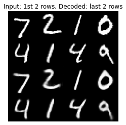
- 인코더 모델은 낮은 차원의 잠재 벡터를 생성하기 위해서 Conv2D(32)-Conv2D(64)-Dense(16)으로 구성
- 디코더 모델은 Dense(16)-Conv2DTranspose(64)-Conv2DTranspose(32)-Conv2DTranspose(1)으로 구성
- 입력은 원본 입력을 복원하기 위한 디코딩된 잠재 벡터
잠재벡터 시각화

- 잠재 코드 차원
- 숫자 0: 왼쪽 아래 사분면
- 숫자 1: 오른쪽 위 사분면
노이즈 제거 오토인코더(DAE)
노이즈 제거 Denoising
\[ x = x_{orig} + noise \]
인코더의 목적: 잠재벡터인 \(z\)를 생성하는 방법을 찾는 것 \(\to\) 잠재 벡터를 디코더가 MSE와 같은 손실 함수의 비 유사성을 최소화하여 \(x_{orig}\)로 복원
\[ L(x_{orig}, \tilde{x}) = MSE = \frac{1}{m} \sum _{i=1} ^{i=m} (x _{origi} - {\tilde{x _{i}}} ) ^{2}\]
'''Trains a denoising autoencoder on MNIST dataset.

Denoising is one of the classic applications of autoencoders.
The denoising process removes unwanted noise that corrupted the
true data.

Noise + Data ---> Denoising Autoencoder ---> Data

Given a training dataset of corrupted data as input and
true data as output, a denoising autoencoder can recover the
hidden structure to generate clean data.

This example has modular design. The encoder, decoder and autoencoder
are 3 models that share weights. For example, after training the
autoencoder, the encoder can be used to  generate latent vectors
of input data for low-dim visualization like PCA or TSNE.
'''

from __future__ import absolute_import
from __future__ import division
from __future__ import print_function

from tensorflow.keras.layers import Dense, Input
from tensorflow.keras.layers import Conv2D, Flatten
from tensorflow.keras.layers import Reshape, Conv2DTranspose
from tensorflow.keras.models import Model
from tensorflow.keras import backend as K
from tensorflow.keras.datasets import mnist
import numpy as np
import matplotlib.pyplot as plt
from PIL import Image

np.random.seed(1337)

# load MNIST dataset
(x_train, _), (x_test, _) = mnist.load_data()

# reshape to (28, 28, 1) and normalize input images
image_size = x_train.shape[1]
x_train = np.reshape(x_train, [-1, image_size, image_size, 1])
x_test = np.reshape(x_test, [-1, image_size, image_size, 1])
x_train = x_train.astype('float32') / 255
x_test = x_test.astype('float32') / 255

# generate corrupted MNIST images by adding noise with normal dist
# centered at 0.5 and std=0.5
noise = np.random.normal(loc=0.5, scale=0.5, size=x_train.shape)
x_train_noisy = x_train + noise
noise = np.random.normal(loc=0.5, scale=0.5, size=x_test.shape)
x_test_noisy = x_test + noise

# adding noise may exceed normalized pixel values>1.0 or <0.0
# clip pixel values >1.0 to 1.0 and <0.0 to 0.0
x_train_noisy = np.clip(x_train_noisy, 0., 1.)
x_test_noisy = np.clip(x_test_noisy, 0., 1.)

# network parameters
input_shape = (image_size, image_size, 1)
batch_size = 32
kernel_size = 3
latent_dim = 16
# encoder/decoder number of CNN layers and filters per layer
layer_filters = [32, 64]

# build the autoencoder model
# first build the encoder model
inputs = Input(shape=input_shape, name='encoder_input')
x = inputs

# stack of Conv2D(32)-Conv2D(64)
for filters in layer_filters:
    x = Conv2D(filters=filters,
               kernel_size=kernel_size,
               strides=2,
               activation='relu',
               padding='same')(x)

# shape info needed to build decoder model so we don't do hand computation
# the input to the decoder's first Conv2DTranspose will have this shape
# shape is (7, 7, 64) which can be processed by the decoder back to (28, 28, 1)
shape = K.int_shape(x)

# generate the latent vector
x = Flatten()(x)
latent = Dense(latent_dim, name='latent_vector')(x)

# instantiate encoder model
encoder = Model(inputs, latent, name='encoder')
encoder.summary()

# build the decoder model
latent_inputs = Input(shape=(latent_dim,), name='decoder_input')
# use the shape (7, 7, 64) that was earlier saved
x = Dense(shape[1] * shape[2] * shape[3])(latent_inputs)
# from vector to suitable shape for transposed conv
x = Reshape((shape[1], shape[2], shape[3]))(x)

# stack of Conv2DTranspose(64)-Conv2DTranspose(32)
for filters in layer_filters[::-1]:
    x = Conv2DTranspose(filters=filters,
                        kernel_size=kernel_size,
                        strides=2,
                        activation='relu',
                        padding='same')(x)

# reconstruct the denoised input
outputs = Conv2DTranspose(filters=1,
                          kernel_size=kernel_size,
                          padding='same',
                          activation='sigmoid',
                          name='decoder_output')(x)

# instantiate decoder model
decoder = Model(latent_inputs, outputs, name='decoder')
decoder.summary()

# autoencoder = encoder + decoder
# instantiate autoencoder model
autoencoder = Model(inputs, decoder(encoder(inputs)), name='autoencoder')
autoencoder.summary()

# Mean Square Error (MSE) loss function, Adam optimizer
autoencoder.compile(loss='mse', optimizer='adam')

# train the autoencoder
autoencoder.fit(x_train_noisy,
                x_train,
                validation_data=(x_test_noisy, x_test),
                epochs=10,
                batch_size=batch_size)

# predict the autoencoder output from corrupted test images
x_decoded = autoencoder.predict(x_test_noisy)

# 3 sets of images with 9 MNIST digits
# 1st rows - original images
# 2nd rows - images corrupted by noise
# 3rd rows - denoised images
rows, cols = 3, 9
num = rows * cols
imgs = np.concatenate([x_test[:num], x_test_noisy[:num], x_decoded[:num]])
imgs = imgs.reshape((rows * 3, cols, image_size, image_size))
imgs = np.vstack(np.split(imgs, rows, axis=1))
imgs = imgs.reshape((rows * 3, -1, image_size, image_size))
imgs = np.vstack([np.hstack(i) for i in imgs])
imgs = (imgs * 255).astype(np.uint8)
plt.figure()
plt.axis('off')
plt.title('Original images: top rows, '
          'Corrupted Input: middle rows, '
          'Denoised Input:  third rows')
plt.imshow(imgs, interpolation='none', cmap='gray')
Image.fromarray(imgs).save('corrupted_and_denoised.png')
plt.show()
Model: "encoder"
_________________________________________________________________
Layer (type) Output Shape Param #
=================================================================
encoder_input (InputLayer) [(None, 28, 28, 1)] 0
conv2d_4 (Conv2D) (None, 14, 14, 32) 320
conv2d_5 (Conv2D) (None, 7, 7, 64) 18496
flatten_2 (Flatten) (None, 3136) 0
latent_vector (Dense) (None, 16) 50192
=================================================================
Total params: 69,008
Trainable params: 69,008
Non-trainable params: 0
_________________________________________________________________
Model: "decoder"
_________________________________________________________________
Layer (type) Output Shape Param #
=================================================================
decoder_input (InputLayer) [(None, 16)] 0
dense_2 (Dense) (None, 3136) 53312
reshape_2 (Reshape) (None, 7, 7, 64) 0
conv2d_transpose_4 (Conv2DT (None, 14, 14, 64) 36928
ranspose)
conv2d_transpose_5 (Conv2DT (None, 28, 28, 32) 18464
ranspose)
decoder_output (Conv2DTrans (None, 28, 28, 1) 289
pose)
=================================================================
Total params: 108,993
Trainable params: 108,993
Non-trainable params: 0
_________________________________________________________________
Model: "autoencoder"
_________________________________________________________________
Layer (type) Output Shape Param #
=================================================================
encoder_input (InputLayer) [(None, 28, 28, 1)] 0
encoder (Functional) (None, 16) 69008
decoder (Functional) (None, 28, 28, 1) 108993
=================================================================
Total params: 178,001
Trainable params: 178,001
Non-trainable params: 0
_________________________________________________________________
Epoch 1/10
1875/1875 [==============================] - 11s 6ms/step - loss: 0.0367 - val_loss: 0.0205
Epoch 2/10
1875/1875 [==============================] - 11s 6ms/step - loss: 0.0193 - val_loss: 0.0180
Epoch 3/10
1875/1875 [==============================] - 11s 6ms/step - loss: 0.0176 - val_loss: 0.0172
Epoch 4/10
1875/1875 [==============================] - 11s 6ms/step - loss: 0.0168 - val_loss: 0.0166
Epoch 5/10
1875/1875 [==============================] - 11s 6ms/step - loss: 0.0163 - val_loss: 0.0163
Epoch 6/10
1875/1875 [==============================] - 11s 6ms/step - loss: 0.0160 - val_loss: 0.0161
Epoch 7/10
1875/1875 [==============================] - 11s 6ms/step - loss: 0.0157 - val_loss: 0.0160
Epoch 8/10
1875/1875 [==============================] - 11s 6ms/step - loss: 0.0154 - val_loss: 0.0160
Epoch 9/10
1875/1875 [==============================] - 11s 6ms/step - loss: 0.0153 - val_loss: 0.0157
Epoch 10/10
1875/1875 [==============================] - 11s 6ms/step - loss: 0.0151 - val_loss: 0.0156
313/313 [==============================] - 1s 2ms/step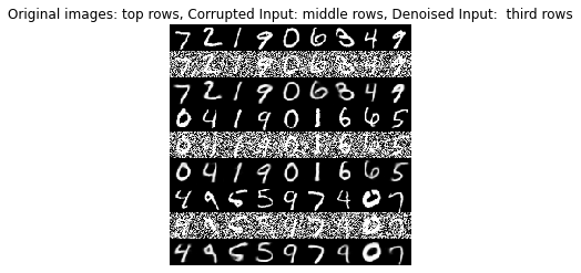
자동 채색 오토인코더
해당 코딩은 너무 길어서 생략. 자세한 것은 여기 링크 참고 \(\to\) 자동 채색 오토인코더
입력: 회색도 사진, 출력: 해당하는 채색된 사진들로 오토인코더를 훈련

요약
- 노이즈 제거, 채색 등 구조적인 변환을 효율적으로 하기 위하여 데이터를 낮은 차원의 표현으로 압축하는 신경망
4장 생성적 적대 신경망(GAN)
- 생성자(generator): 판별자를 속일 수 있는 가짜 데이터 신호를 생성하는 방법에 대해 지속적으로 알아내는 것
- 판별자(discriminator): 가짜와 실제 신호를 구분하도록 훈련
- 유요한 데이터는 1.0으로 레이블링 되고 합성된 데이터는 0.0(진짜일 확률 0%)로 레이블ㄹ이 된다.
생성기 개발을 위한 클래스
class Generator:

    def __init__(self):
        self.initVariable = 1

    def lossFunction(self):

        return

    def buldModel(self):

        return

    def trainModel(self, inputX, inputY):

        return
판별기 개발을 위한 클래스
class Discriminator:

    def __init__(self):
        self.initVariable = 1

    def lossFunction(self):

        return

    def buildModel(self):

        return

    def trainModel(self,inputX,inputY):

        return
손실 함수
class Loss:

    def __init__(self):
        self.initVariable = 1

    def lossBaseFunction1(self):

        return

    def lossBaseFunction2(self):

        return


    def lossBaseFunction3(self):

        return
- 적대적 훈련을 할 때 생성기에서 사용하는 손실함수
\[\nabla \theta_g \sum_{i=1}^{m} log(1-D(G(z^{(i)}))) \]
- GAN에서 적용되는 표준 교차 엔트로피 구현
\[ \nabla \theta_d \dfrac{1}{m} \sum_{i=1}^{m} [logD(x^{(i)})+log(1-D(G(z^{(i)})))] \]
- 굿펠로우 논문에 나오는 함수
note: 교수님이 설명해주신 코드 보는게 더 나을듯 하다. 교수님 코드
DCGAN
- 심층 CNN을 이용하여 초기 GAN를 성공적으로 구현
조건부(Conditional) GAN
- 원-핫 벡터를 제외하면 DCGAN과 유사
- 생성자와 판별자의 출력에 조건을 부여하기 위해 원-핫 벡터 사용
5장 향상된 GAN
Wasserstein GAN
GAN의 불안정성은 Jensen-Shannon (JS) 거리에 기초한 손실함수 때문이라고 주장
GAN의 최적화에 더 알맞게 JS거리 함수를 대체하기에 적합한 것을 찾아야함
ref: https://lilianweng.github.io/posts/2017-08-20-gan/
- 책 개념이 너무 어렵당.. 관련 수식에 대해 이해하고 싶은뎀 수식에 대한 내용이 자세하진 않음.. 일단 수식에 대한 내용이해 먼저 하고 추후에 다시 책 읽어보는 걸로~~